Benchmarking Julia on the 2d Heat Equation

Abstract

In scientific computation, programming languages must enable high programmer productivity without sacrificing performance. The Julia programming language follows a novel approach utilizing a just-in-time compiler to provide performance comparable to low-level languages like C or C++ in a syntax similar to high-level scripting languages like Python. Its LLVM backend allows compiling Julia code for CPU and GPU. In this work, we explore how the performance of Julia code in different programming styles compares to Numpy, PyTorch, C++, and CUDA-C implementations of a typical structured grid stencil code. We measure throughput similar to or superior to C++ for CPU and GPU computations. The syntax of array-based computations in Julia closely resembles Python’s Numpy and PyTorch but offers significantly better performance. When working with stencil codes, Julia outperforms Python by several orders of magnitude on our test problem.

I Introduction

As modern HPC systems have entered the exascale era, programming those systems to achieve maximum performance becomes an ever greater challenge. Long over are the days of Dennard scaling, when regular increases in clock frequency made possible by more miniaturized processes made general-purpose CPUs significantly faster every year. Nowadays, to get more compute power, it is necessary to use multicore processors and accelerators[12]. Writing code that maps parallel tasks to parallel hardware resources is essential to effectively utilize those resources.

High-level languages with automatic parallelization promise a solution to the loss of programmer productivity caused by having to implement explicit parallelism in low-level languages. The Julia programming language stands out among the high-level languages that have entered the scene in recent years. It offers similar high-level expressiveness as interpreted languages like Python while claiming to be capable of execution as fast as highly optimized low-level C code. This performance is enabled by a Just-In-Time compiler based on the LLVM compiler infrastructure with a powerful automatic optimizer.

LLVM can not only target CPUs but can also be used to generate code for a selection of accelerators. For Julia, there exists the CUDA.jl package, which, like the CUDAnative.jl and CUArrays.jl packages that preceded it, enables targeting Julia code for execution on Nvidia General Purpose GPUs (GPGPU) supporting Nvidia’s Compute Unified Device Architecture (CUDA)[2]. In an HPC landscape where efficient and productive utilization of accelerators is critical to competitive performance, the value of a language like Julia is evident, which promises code reuse across different classes of devices at no performance cost.

In this work, we evaluate the performance of Julia and competing programming languages in a simple scientific computing benchmark. As our test problem, we choose time-stepping in a transient 2D heat transfer problem. The problem, a Poisson equation, and our implementation, a stencil code (or its abstractions), represent structured grid problems with applications in fluid dynamics, structural mechanics, and thermal simulations.

We will compare the performance of different implementations of the sample application in other programming languages and styles. We especially want to compare different flavors of Julia programming to conceptually similar languages and the competition in the HPC space. Python offers even more abstraction at the cost of the slow performance of an interpreted language. Of interest to us are the NumPy and PyTorch libraries for Python. These libraries also cover the field of numerical calculations by adding to the Python language array types that precompiled kernels can be applied to. CUDA-C sits at the other extreme, trading high-level programming comforts for low-level control over code execution.

II Preliminaries

II-A Julia in HPC

The Julia programming language is designed with high-performance computing in mind. Its goal is to provide a high-level programming language that is as fast as low-level languages like C or Fortran. The approach taken by the Julia developers is to use a Just-In-Time (JIT) compiler based on the LLVM compiler infrastructure [3]. This allows to generate optimized machine code without relying on bindings to external libraries written in low-level languages such as NumPy for Python [6]. While this approach enables performance that is on par with C for specific problems, it comes at the cost of a startup time for the JIT compiler, known as the ”time to first plot” problem. A significant effort from the side of the Julia developers has reduced this time from around 10s for the first plot in version 1.6 to less than 2s in version 1.10 by caching the compiled code.

Further, Julia can compile to GPU code for Nvidia, AMD, Intel, and Apple GPUs. The respective packages, CUDA.jl, AMDGPU.jl, oneAPI.jl, and Metal.jl, define an array type that is backed by GPU memory and can be used in the same way as regular arrays. This includes element-wise operations, reductions, and linear algebra operations. For more complex operations, the packages allow to write custom kernels in Julia that are compiled to GPU code. Any Julia code that does not dynamically allocate memory is supported here [2]. The CUDA.jl package is the most mature of the four and is used in this work to evaluate the performance of Julia on Nvidia GPUs.

Previous analyses of Julia claim positive performance results. The authors of Julia claim to achieve performance comparable to C in various numerical micro-benchmarks on the CPU using high-level code [3]. Similar results have been reported for GPU code using the CUDA.jl package, with performance of $\pm 5\%$ compared to CUDA-C using significantly fewer lines of code [2]. A specialized investigation finds a speedup from 20x to 100x for solving ODEs on various GPU architectures using Julia [13].

II-B Numerical computations in Python

NumPy is a Python library for performing numerical calculations with the ease of use of the dynamically typed, interpreted Python scripting language. The programming model of NumPy is very similar to the Julia programming language, with many of the same features like array slicing[5]. Because it is very similar in the programming features it provides, NumPy is an interesting point of comparison for Julia.

PyTorch is a deep learning framework that allows the Torch tensor library to be interfaced with Python. This is accomplished through the pytorchlib backend, written in C++, that allows for efficient calculations on both CPU and GPUs. Despite deep learning being its main focus, the PyTorch library provides a fully-featured suite of tools for numerical computation[11]. What makes PyTorch interesting to compare with Julia is how it enables the expression of numerical algorithms for the GPU on a very high level of abstraction. With the increasing importance of differentiable physics for physics deep learning, frameworks like PyTorch also see use for implementing differentiable PDE solvers[7].

II-C Our test problem

We discretize the transient 2D heat equation with a finite difference scheme on a regular grid. A parabolic partial differential equation describes the heat distribution in a given region over time. For a domain $\mathrm{\Omega }=[0,1]\times [0,1]$, a time interval $[0,T]$, and a temperature distribution $u(x,y,t)$, the heat equation reads

${\displaystyle \frac{\partial u}{\partial t}}$ $={\nabla }^{2}u$ (1)

$u(x,y,t=0)$ $=1\forall x,y\in (0,1)$ (2)

$u(x,y,t)$ $=0\forall t\text{for}x=0,x=1,y=0,y=1$ (3)

We discretize the spatial domain with a regular grid of $N\times N$ points and the time domain with a time step $\mathrm{\Delta }t$. We use a second-order finite difference scheme to approximate the Laplacian operator and explicit Euler time stepping. This results in the following numerical scheme:

$u_{i,j}^n$ $\approx u(x_i,y_j,t_n)$ (4)

$x_i$ $=i\cdot h$ (5)

$y_j$ $=j\cdot h$ (6)

$t_n$ $=n\cdot \mathrm{\Delta }t$ (7)

$h$ $={\displaystyle \frac{1}{N-1}}$ (8)

$u_{i,j}^{n+1}$ $=u_{i,j}^n+{\displaystyle \frac{\mathrm{\Delta }t}{h^2}}\cdot (u_{i+1,j}^n+u_{i-1,j}^n+u_{i,j+1}^n+u_{i,j-1}^n$

$-4\cdot u_{i,j}^n)$ (9)

$u_{i,j}^0$ $=1$ (10)

$u_{i,j}^n$ $=0\text{for}i=0,i=N,j=0,j=N$ (11)

Von Neumann stability analysis shows that the explicit Euler scheme is stable for $\mathrm{\Delta }t\le \frac{h^2}{4}$ [9, chapter 5.2].

II-D Implementation techniques

We implement the discretization using two classes of implementation techniques: stencil codes and array codes.

Stencil codes closely resemble the mathematical description of the problem from Eq. 4, as shown in Algorithm 1. They work on a 2d array $u\in {ℝ}^{N+1\times N+1}$, representing the temperature values at the grid points. The grid points at the domain’s boundaries are not updated, enforcing the Dirichlet boundary conditions. The update of the interior grid points is expressed in a nested loop over the grid points, where the new value of a grid point is computed from the values of its neighbors. After each iteration, $u$ is set to $u_{new}$. Here, memory allocations can be avoided by swapping the pointers of $u$ and $u_{new}$, making the old values the buffer for the next values of the next iteration.

Data: $N$, $T$, $\mathrm{\Delta }t$

Result: $y=x^n$

Initialize $u,u_{\text{new}}$ as $(N+1)\times (N+1)$ arrays;

Set $u[1:N,1:N]\leftarrow 1$, $u[0,:],u[N,:],u[:,0],u[:,N]\leftarrow 0$;

$h\leftarrow 1/(N-1)$;

forall $t\in 0:\mathrm{\Delta }t:T$ do

       forall $i\in 1:(N-1)$ do

             forall $j\in 1:(N-1)$ do

                   $u_{\text{new}}[i,j]\leftarrow u[i,j]+\frac{\mathrm{\Delta }t}{h^2}\cdot (u[i+1,j]+u[i-1,j]+u[i,j+1]+u[i,j-1]-4\cdot u[i,j])$;

                  

             end forall

            

       end forall

      $u,u_{\text{new}}\leftarrow u_{\text{new}},u$;

      

end forall

Algorithm 1 Stencil discretization of heat equation

Array codes use the array abstraction to express the computation. $u[a:b,c:d]$ returns a subarray of $u$ with the indices $[a,b)$ in the first dimension and $[c,d)$ in the second dimension. This subarray may be implemented as a view, avoiding memory allocations. Compared to the stencil codes, the compiler has more control of the order of operations. Stencil codes process each grid point individually, loading the values of its neighbors from memory. Array codes, on the other hand, declare the update of all grid points as an expression on all left, right, top, and bottom neighbors, as shown in Algorithm 2.

Data: $N$, $T$, $\mathrm{\Delta }t$

Result: $y=x^n$

Initialize $u$ as $(N+1)\times (N+1)$ arrays;

Set $u[1:N,1:N]\leftarrow 1$, $u[0,:],u[N,:],u[:,0],u[:,N]\leftarrow 0$;

$h\leftarrow 1/(N-1)$;

forall $t\in 0:\mathrm{\Delta }t:T$ do

       $top\mathrm{\_}nbrs\leftarrow u[2:N+1,1:N]$;

       $left\mathrm{\_}nbrs\leftarrow u[1:N,0:N-1]$;

       $right\mathrm{\_}nbrs\leftarrow u[1:N,2:N+1]$;

       $bottom\mathrm{\_}nbrs\leftarrow u[0:N-1,1:N]$;

       $self\leftarrow u[1:N,1:N]$;

       $u[1:N,1:N]\leftarrow self+\frac{\mathrm{\Delta }t}{h^2}\cdot (top\mathrm{\_}nbrs+left\mathrm{\_}nbrs+right\mathrm{\_}nbrs+bottom\mathrm{\_}nbrs-4\cdot self)$;

      

end forall

Algorithm 2 Array discretization of heat equation

III Methodology

III-A Implementation Details

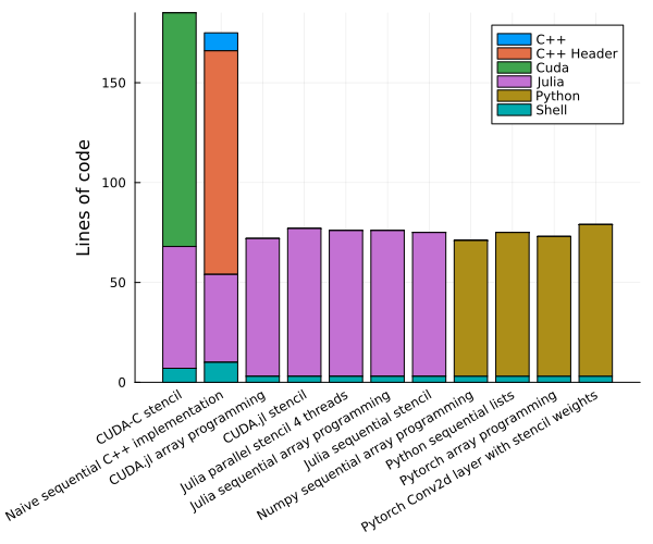
We implement the discretization of the heat equation in Python, C++, and Julia with different programming styles as summarized in Table I. The implementations are available in this repository. All implementations are relatively small (see Fig. 1) and allow writing to the vtk format for visualization.

Name	Programming Language	Hardware	Programming Style	Compiler	Precision
C++ naive baseline	C++	CPU	Kernel	GCC 9.3	Double
julia sequential array programming	Julia	CPU	Array	Julia 1.10	Double
Julia sequential stencil	Julia	CPU	Stencil	Julia 1.10	Double
Julia parallel stencil	Julia	CPU (multithreaded)	Stencil	Julia 1.10	Double
Python sequential lists	Python	CPU	Stencil	Python 3.8	Double
NumPy sequential array programming	Python (NumPy)	CPU	Array	Python 3.8, NumPy 1.23	Double
CUDA-C stencil	C++	GPU (CUDA)	Stencil	NVCC 22	Single
CUDA.jl stencil	Julia	GPU (CUDA)	Stencil	Julia 1.10	Single
CUDA.jl array programming	Julia	GPU (CUDA)	Array	Julia 1.10	Single
Pytorch array programming	Python (PyTorch)	GPU (CUDA)	Array	Python 3.8, torch 2.3	Single
Pytorch conv	Python (PyTorch)	GPU (CUDA)	CNN	Python 3.8, torch 2.3	Single

TABLE I: Implementations studied in this work. Available in this repository.

Figure 1: Lines of code by implementation. The C++ implementations require about twice as many lines of code as the high-level languages. Further, the C++ implementations are not able to write to the vtk format, which is why we add glue code to convert from a simple text format to vtk.

III-A1 C++ Reference

As the baseline for our performance analysis, we use a naive sequential implementation in C++, being the de facto standard for HPC applications. Our implementation represents the temperature field as a vector of vectors and closely follows Algorithm 1. While the discretization logic is straightforward to implement, all I/O operations and the compilation process are significantly more complex in C++ than in high-level languages. Writing to the vtk format proved to be especially challenging, prompting us to write a simple text format that we convert to vtk using a Julia script.

III-A2 Julia CPU Code

We implement two base versions of the code, one using array programming and one applying a stencil. The array programming implementation is not parallelized. Memory allocations are avoided using the @views macro. The implementation follows the array code in Algorithm 2.

The stencil code is parallelized using the Threads.@threads macro with a static schedule. The static schedule is essential because the 128MB of L3 cache of the AMD 7402 is divided into different NUMA regions, so a consistent mapping of loop iterations to processors boosts performance.

We also turned off bounds checking in the Julia code for a fair comparison with the C++ code.

The Julia code is significantly shorter than the C++ code and more concise due to features like native multi-dimensional arrays, array slicing, a package manager with a rich ecosystem, and a powerful standard library.

III-A3 Julia GPU Code

Porting the array code to the GPU is straightforward using the CUDA.jl package since the CuArray type follows the same interface as the regular Array type.

The stencil code is implemented as a custom kernel. It is launched with a 2D grid and a 2D block using the CUDA.@cuda macro with a block size of $8\times 8$ threads. Copying data between CPU and GPU is completely avoided unless results are saved to disk. We use single-precision floating-point numbers for all GPU implementations to exploit optimized hardware support.

The most significant difference between the CPU and GPU implementations in terms of code is that all GPU functionality must be written in a separate function. Further, a less mature compiler infrastructure on the GPU impacts the developer experience compared to the CPU. While the JIT compilation takes less than two seconds on the CPU, delays of up to 15 seconds are typical for GPU code. Moreover, error messages are less informative and more challenging to debug.

III-A4 C++ CUDA

We represent the temperature field as a 1D array and use CUDA with NVCC to parallelize the stencil computation. Similar to the Julia GPU implementation, we use a 2D grid and a 2D block of $8\times 8$ threads and avoid copying data between CPU and GPU. Ergonomics are even slightly worse than those with naive C++ since using low-level CUDA primitives is necessary, and the compilation process is more complex.

III-A5 Python

The Python stencil code represents the temperature field as a list of lists and closely follows Algorithm 1.

We implement array code with both torch and NumPy. While the NumPy implementation is single-threaded, the torch implementation uses the GPU for computation. Gradient computation is disabled to avoid unnecessary overhead.

Further, we implement a GPU-accelerated stencil code using a convolutional neural network (CNN) with PyTorch. The CNN has a single convolutional layer with a kernel size of $3\times 3$ and weights of $[[0,1,0],[1,-4,1],[0,1,0]]$.

For this simple problem, ergonomics and lines of code are very similar between the Python and Julia implementations. However, both NumPy and PyTorch rely on array programming to achieve acceptable performance, potentially limiting flexibility for more complex challenges.

III-B Experimental setup

We discretize the domain with spatial resolutions of $N\in \{100,200,400,800,1600,3200,6400,12800\}$ for $5000$ time steps. The time step size is chosen to fulfill the stability criterion (see Section II-C). We benchmark the runtime of the different implementations using the BenchmarkTools.jl package in Julia and custom scripts in Python and C++ [4]. The runtime includes the initialization of the domain and the time stepping but excludes compilation time and does not write the results to disk. We measure the runtime of the different implementations and calculate the speedup compared to the naive C++ implementation. If an implementation is significantly slower than the naive C++ implementation, we run it for fewer steps to reduce the runtime and correct it accordingly.

III-C Test environment

We measure the performance of our code on an AMD Zen2-based server running Ubuntu 20.04.02 LTS, Linux kernel version 5.4.0-81. We measure the wall clock time needed to complete 5000 iterations for every scenario with disabled output. The baseline for all speedup numbers is the performance of the naive C++ implementation compiled with gcc and optimization level -O3.

The system’s processor is an AMD EPYC 7402 24-core CPU operating at 2.8GHz. Eight channels of DDR4-3200 DRAM provide a main memory bandwidth of 204.8GB/s, and the shared L3 cache is 128MB in size. Every core can perform up to four floating-point operations on 128-bit vectors per cycle, but some restrictions apply; for example, only two units are capable of Fused-Multiply-Add (FMA). The theoretical peak vector performance of the whole processor is 768 FLOP/cycle in single precision and 384 double precision operations per cycle. This gives a peak performance of 2.15 TFLOP/s for single precision and 1.075 TFLOP/s for double precision. Hyperthreading is available on the system but was not used because our stencil computation is memory-bound, so it would not benefit from more efficient utilization of compute units.

The GPUs we used for testing are RTX 3080s (10GB version) from the Ampere generation of Nvidia GPUs. There are four identical GPUs on the system, but our application only uses one of them. This version of the RTX 3080 has 8704 CUDA Cores on 68 streaming multiprocessors. The theoretical peak performance is 29.77TFLOP/s in single precision and 465GFLOP/s in double precision. The ten gigabytes of video RAM are connected to the GPU through a 320-bit wide bus with a maximum memory bandwidth of 760.3GB/s[10].

IV Performance Analysis

IV-A Challenges to achieving good performance

Our example problem, the heat equation discretized using a five-point stencil, is inherently hard to perform efficiently on parallel hardware because of the low arithmetic intensity inherent to structured grid stencil computations. There are rapidly diminishing returns when adding more compute power to the problem without adding additional memory bandwidth, for example by utilizing more nodes with their individual memories and memory interfaces.

For every domain element, we perform four additions, one subtraction, and two multiplications with constants that can be precomputed and stored in registers. The multiplications can be fused with the subtraction and one of the additions into fused multiply-add (FMA) operations so that five floating point operations are performed per element. Five values need to be loaded from memory, and the result must be stored at a different location for every element.

Modern hardware is much faster at performing computations than at loading data from main memory. With every generation of hardware, the gap between compute and memory speed widens; this is called the memory wall[8]. The effective use of the caches is critical to achieving good performance despite the memory wall. For our example code, how well it utilizes the caches depends on the domain size. Small domains can ideally be entirely stored in the cache, while larger domains can not fit whole rows into the fastest caches. Even if no whole row of domain cells fits into the cache, if cells are processed sequentially and the values are stored contiguously in memory, two of the five values that must be loaded can be read from the cache (except at the start of a row).

Figure 2: Speedup for different domain sizes on the CPU compared to the naive C++ implementation. The shaded area indicates $1\sigma$ confidence intervals. The implementations are run once for larger domain sizes due to resource constraints, so no confidence intervals are shown.

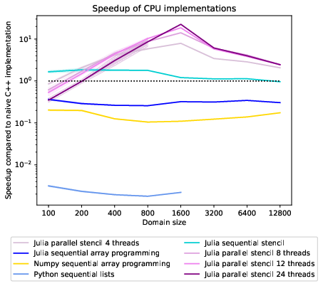
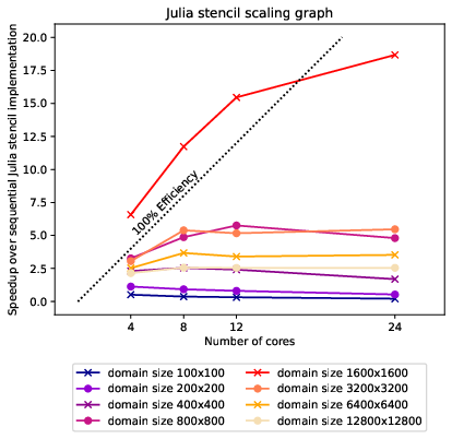
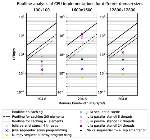
From the speedup graph 2 comparing the performance of our implementations on different domain sizes, we can tell that the best performance is achieved at a domain size of 1600x1600. In the scaling graph in figure 3, we can see that this configuration even achieves superlinear speedup compared to the sequential Julia stencil implementation. The scaling graph in figure 3 shows four processors give $6.6$ times speedup at a parallel efficiency of $160\%$. The superlinear speedup is achieved because the sequential implementation can not fit the 20MB domain into the most easily accessible L3 cache. In the AMD Zen 2 architecture, a Core Complex Die (CCD) contains two NUMA domains with 16MB of L3 cache for each Core Complex (CCX)[1]. The local domains of the multi-threaded approach fit into the L3 cache of a CCX. We do not see super-linear speedup for the smaller domain size of 800x800 because, for that domain size, the L3 cache of one CCX suffices to store the whole domain, so the sequential performance is better, an observation we can also make in the GFlop/s graph 4. The drop in performance of the sequential stencil implementation relative to the C++ implementation between the 800x800 and the 1600x1600 domain is probably caused by the L3 cache being unable to serve the fast memory accesses needed for vectorization to give a performance uplift.

Figure 3: Plot of speedup over core count in the Julia parallel stencil code. The baseline is the sequential stencil computation in Julia.

Figure 4: FLOP/s for different domain sizes on the CPU. The shaded area indicates $1\sigma$ confidence intervals. The implementations are run once for larger domain sizes due to resource constraints, so no confidence intervals are shown.

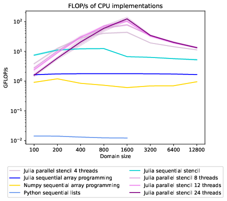
The arithmetic intensity of the problem for double precision floats is $\frac{5}{48}\frac{FLOP}{bytes}$ if no caching takes place at all. In this scenario, the code would be compute bound up to a memory bandwidth above $1075\frac{GFLOP}{s}\cdot \frac{48}{5}\frac{byte}{FLOP}=10320\frac{GB}{s}$, more than 50 times the memory bandwidth available on the test system. Our expected performance would be $204.8\frac{GB}{s}\cdot \frac{5}{48}$ The implementations are run once for larger domain sizesThe implementations are run once for larger domain sizes $\frac{FLOP}{bytes}$ = 21.3 $\frac{GFLOP}{s}$, most implementations perform better than that, so there is a positive effect from caching. With caching of two elements, like when no whole row fits in the cache, the arithmetic intensity is $\frac{5}{32}\frac{FLOP}{bytes}$, the expected performance is $32\frac{GFLOP}{s}$.

The roofline plot shows that the multithreaded implementations perform above the roofline for successfully caching one or two elements needed for the five-point stencil. This indicates that for the domain size 1600x1600, caching enables performance beyond what is achievable with only main memory accesses. At the optimal domain size, the stencil implementation on 24 cores almost hits the maximum performance considering the remaining memory access, storing the result.

IV-B Performance comparison of CPU implementations

The best-performing implementation is the Julia stencil code running on all 24 cores on a domain of 1600x1600. For larger domains, more than eight cores do not give additional performance benefits. The sequential Julia stencil implementation performs better for smaller domain sizes than the naive C++ implementation. Because Julia arrays are guaranteed not to alias, unlike C pointers, it might be that the Julia code is vectorized more efficiently. For larger domain sizes, where slower caches and main memory serve more accesses, the sequential Julia stencil and C++ implementations perform almost identically.

Array programming for sequential Julia CPU code can not compete with naive C++ programming but still outperforms the Numpy array programming implementation. In Julia, we communicated our intent of using the values from the array slices without creating copies of the arrays by using the @views macro. In NumPy, slicing operations create views, not copies, by default, so the lower performance of NumPy can not be explained by additional copies being produced. For this application, Julia is far superior to Numpy, with an order of magnitude higher performance of the stencil code than the NumPy array code.

Figure 5: Multi-threaded Julia code achieves almost ideal performance according to the roofline model for domain size 1600x1600. For smaller and larger domain sizes, actual performance is an order of magnitude below the theoretical limit imposed by memory access speed.

IV-C Performance comparison of GPU implementations

Performance measurements on the GPU are not directly comparable to CPU performance measurements because of different machine precisions. Current GPUs also offer double precision arithmetic, but usually, they are optimized for single precision, and with newer, AI-focused models, even lower precision operations. While modern CPUs usually achieve half their single precision FLOP/s performance in double precision, our testing GPU, the RTX 3080, has 64 times the single precision FLOP/s peak performance compared to double precision[10]. To provide numbers allowing for comparison between different GPU implementations in the setting the tools were optimized for, we went with single precision for GPU measurements.

Figure 6: Speedup for different domain sizes on the GPU compared to the naive C++ implementation. The shaded area indicates $1\sigma$ confidence intervals. The implementations are run once for larger domain sizes due to resource constraints, so no confidence intervals are shown.

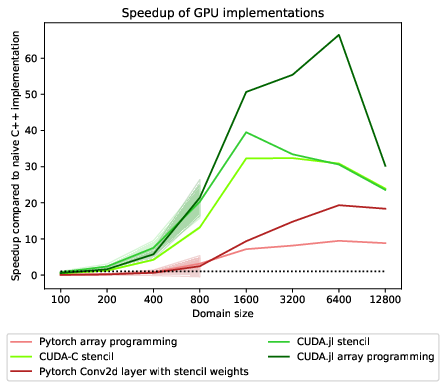
All GPU implementations perform strongly for larger grids but perform poorly for lower resolutions. At 100x100, no GPU implementation in single precision can beat the naive double-precision C++ implementation on the CPU. Partly, this is because of the additional overhead from Kernel launches and the copying of the final result from the device (GPU) to the host (CPU) memory. Another factor is the small domain size, which does not provide the oversubscription necessary for effective latency hiding. At a domain resolution of 100x100, there is only slightly more than one domain cell per CUDA core, so it is impossible to task all SIMD lanes and provide oversubscription. For higher resolutions, all GPU implementations except PyTorch array programming are decisively faster than the fastest CPU implementations, even accounting for the different levels of floating-point precision.

The claim from the paper by Besard et al.[2] was that GPU code written in Julia performs better than or comparable to optimized CUDA-C code. Our measurements can confirm this finding for our toy problem, the 2d heat equation. The Julia kernel code performs slightly better at medium domain sizes than our handwritten CUDA-C kernel. For large domain sizes, they perform almost identically. Significantly improved is the performance of the array programming Julia cuda implementations, which achieves about twice the speedup of the CUDA-C and Julia kernel implementation. We assume that the CUDA-C and Julia Kernel are semantically identical, with an explicit bounds check. This kind of bounds check is typical in human-written CUDA code because threads are commonly launched in equally sized blocks, so it might not be possible to launch threads only for the elements that need to be modified in the array. While the explicit bounds check is usually accepted as a trade-off for duplicate-free code without additional boundary kernels, and an additional kernel incurs additional Kernel launch cost, this area might see optimization by the LLVM optimizing compiler infrastructure.

PyTorch array programming does not perform comparably to custom kernels or array programming in Julia. For larger domain resolutions, using the PyTorch 2d Convolution gives quite good performance with 20 times speedup on the largest domain size, but it is still lagging behind custom stencils. It might be inefficient because the convolution applies a 3x3 filter instead of a five-point stencil. Four additional elements are loaded but do not affect the result because they get multiplied by 0 before the addition. Nevertheless, we are wasting computations by adding elements that are always zero. In strongly memory bandwidth-limited use cases like large domain sizes, we can conclude that PyTorch can offer better performance than CPU implementations but is not competitive with handwritten CUDA Kernels or Julia array programming on the GPU.

V Conclusion

Our results highlight that Julia delivers performance comparable to C++ in a high-level programming language on the scientific stencil computation we benchmarked on the CPU and the GPU. When using array programming, Julia provides ergonomics similar to Numpy or PyTorch at significantly superior performance. However, the real power of the language proved to lie in stencil codes. Here, Julia combines a syntax similar to Python with performance comparable to or superior to C++ on CPU and GPU. When element-wise stencil computations are required, Julia outperforms Python by several orders of magnitude. While the CUDA.jl package delivers strong performance and elegant expressiveness, significant improvements concerning error messages and compilation times are necessary to catch up with the developer experience of the Julia CPU compiler. With these problems solved, Julia could become the go-to language for scientific computing on the GPU, offering high abstraction and productivity without sacrificing performance.

References

- [1] (2019) Advanced micro devices socket sp3 platform numa topology for amd family 17h models 30h–3fh. Technical report Advanced Micro Devices, Inc.. Note: Technical Document External Links: Link Cited by: §IV-A.
- [2] (2018) Effective extensible programming: unleashing Julia on GPUs. IEEE Transactions on Parallel and Distributed Systems. External Links: Document, ISSN 1045-9219, 1712.03112, Link Cited by: §I, §II-A, §II-A, §IV-C.
- [3] (2017) Julia: a fresh approach to numerical computing. SIAM Review 59 (1), pp. 65–98. External Links: Document, Link, https://arxiv.org/abs/1411.1607 Cited by: §II-A, §II-A.
- [4] (2016-08) Robust benchmarking in noisy environments. arXiv e-prints. External Links: 1608.04295 Cited by: §III-B.
- [5] (2020) Array programming with numpy. Nature 585 (7825), pp. 357–362. Cited by: §II-B.
- [6] (2020-09) Array programming with NumPy. Nature 585 (7825), pp. 357–362. External Links: Document, Link Cited by: §II-A.
- [7] (2020) Phiflow: a differentiable pde solving framework for deep learning via physical simulations. In NeurIPS workshop, Vol. 2. Cited by: §II-B.
- [8] (2004) Reflections on the memory wall. In Proceedings of the 1st conference on Computing frontiers, pp. 162. Cited by: §IV-A.
- [9] (2010) Fundamentals of engineering numerical analysis. 2 edition, Cambridge University Press. Cited by: §II-C.
- [10] (2020) NVIDIA ampere ga102 gpu architecture. Technical report NVIDIA Corporation. Note: Whitepaper External Links: Link Cited by: §III-C, §IV-C.
- [11] (2019) PyTorch: an imperative style, high-performance deep learning library. External Links: 1912.01703 Cited by: §II-B.
- [12] (2005) The free lunch is over: a fundamental turn toward concurrency in software. Dr. Dobb’s journal 30 (3), pp. 202–210. Cited by: §I.
- [13] (2024) Automated translation and accelerated solving of differential equations on multiple gpu platforms. Computer Methods in Applied Mechanics and Engineering 419, pp. 116591. External Links: Link Cited by: §II-A.